Using BlendGAMer to Refine a Subcellular Model

Introduction

In this tutorial, you will learn how to use BlendGAMer to generate a tetrahedral mesh suitable for Finite Element computation from a volume electron microscopy (EM) dataset. You will learn how to:

• Import segmented geometries in Blender

• How to use BlendGAMer to improve the quality of the surface mesh

• Use mesh boolean operations to construct a domain of interest

• Generate a tetrahedral mesh with marked domains and boundaries

To complete this tutorial you will need the following installed on your system:

• Blender 2.79b (Download Blender Here)

• BlendGAMer v2.0.3 or later (Getting BlendGAMer)

• (Recommended) three-button mouse

• (Recommended) full size keyboard

Note

We strongly recommend the use of a 3-button mouse and full keyboard with numeric keyboard. While they aren’t strictly necessary, for brevity, this tutorial will present keyboard shortcuts for each step. The locations of menu options corresponding to the shortcuts we leave as an exercise to the user.

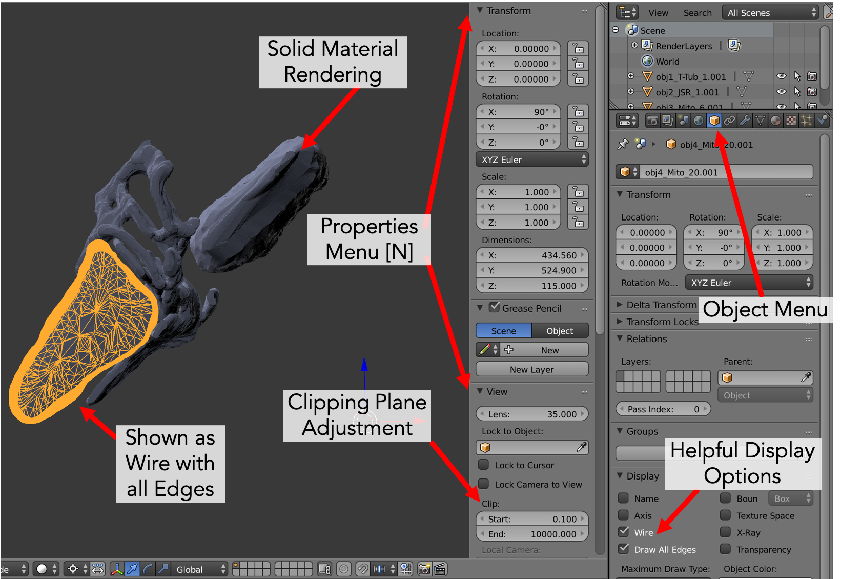
Our model of interest today is the murine cardiac myocyte calcium release unit. You can get the raw electron micrographs and segmentations from the Cell Image Library, a collection of 2D, 3D, and 4D cellular and subcellular data derived from light and electron microscopy. The data we will be using today is from entry 3603. For the purposes of this tutorial, we have selected a nicely segmented section of the dataset for model building, shown in Fig. 7. The software IMOD was used to segment and generate a preliminary mesh in this example.

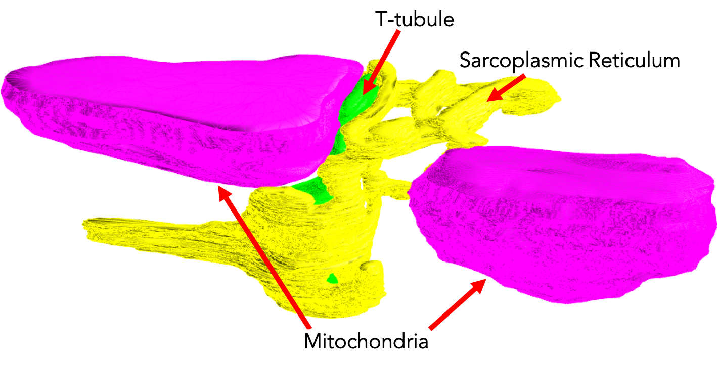
Fig. 7 Components of the scene

Preliminary surface meshes from segmentations are typically of poor quality for computation. A poor quality mesh is broadly defined as one which will lead to large errors in computation or inefficiency. For triangulated surface meshes, the quality of the mesh can be qualitatively judged by visually inspecting the evenness of the edge and vertex distributions. Quantitatively, mesh quality is measured by mesh topology and proportion of high aspect triangles (triangles with extremely large and small angles). A higher quality mesh will contain more equilateral shaped triangles.

Import OBJ File into Blender

Instead of starting with the raw EM data, performing segmentation, and contour tiling, we have already generated an initial mesh for you.

1. Download the obj file. Hint: right click and “Save As” to download as a file.

2. Now we can open up this .obj file in blender.

   • Start Blender. Open the application from the start menu or by typing blender on the command line. You should see something like this.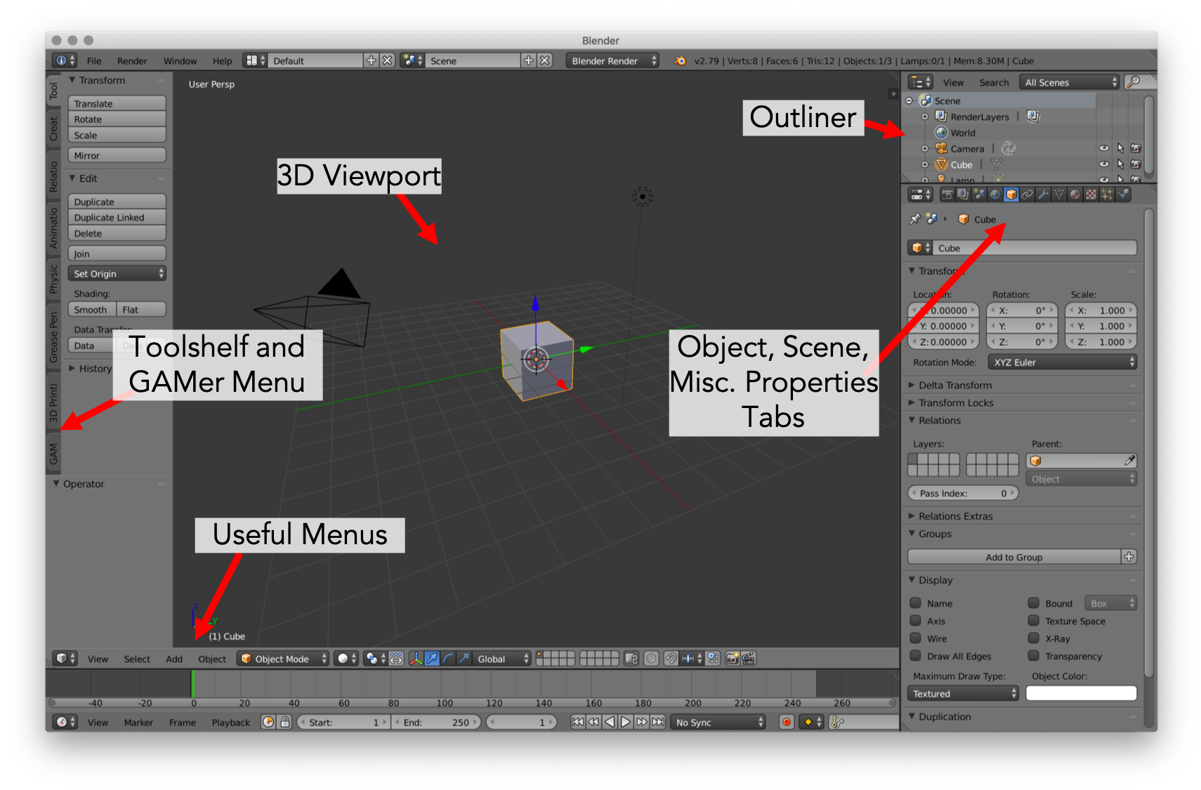

     

     There are several panels and regions in the default Blender interface. Please refer to this if you cannot find a panel in later steps.

   • The Cube, Camera and Lamp are placed in the viewport by default. We won’t need them so go ahead and delete them. Note, Blender has lots of useful keyboard shortcuts. Where applicable in the tutorial, relevant shortcuts are shown as follows: Select All [A], Delete [X].

   • Change the Rotation Mode by going to User Preferences > Input tab > track-ball

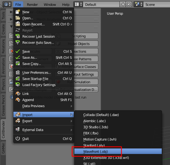
   • Import the data file with File > Import > Wavefront (.obj) and select tt-sr-mit.obj

     

Preliminary Work on Imported Mesh

1. The object is not initially centered around the origin. To bring it into view, do the following:

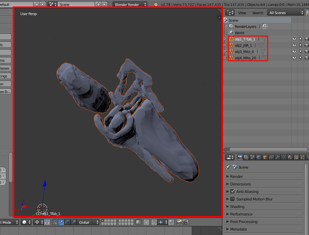
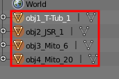
   • Make sure you have all four objects selected by holding shift-LMB and clicking (i.e. left-mouse-button) each object, selected objects will have an orange circle around their respective triangle.

   • With the cursor inside of the 3D view window, press the Period on the Numpad to View > View Selected.

   

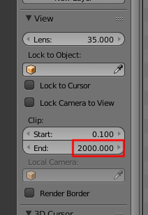
2. You may notice that parts of the model are getting truncated by the clipping plane. To remove the visual artifacts, we can increase the distance of the far clipping pane.

   • Open the Properties panel by having the cursor in the 3D view window and then hitting n.

   • Navigate to the View subpanel.

   • Under Clip, change End to 2000.

   

   • For geometric models, it is often useful to change to the orthographic view [numpad 5].

   

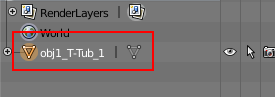
3. We need the model to be in one volumetric domain so let us join it. In the Outliner hold shift-LMB and click (i.e. left-mouse-button) each object with obj1_T-Tub_1 selected last which will appear white.

   

4. Then to join them have the cursor in the 3D view window and press (Ctrl+j), if done correctly then the four objects should combine into obj1_T-Tub_1.

   

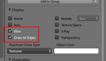
5. The mesh is currently rendered as a solid material. While this is great for the purposes of animation and visualization, we care about the distribution of nodes and edges. To show the edges in the Viewport, go to the Object Properties tab and select Wire and Draw all Edges in the Display subpanel.

   

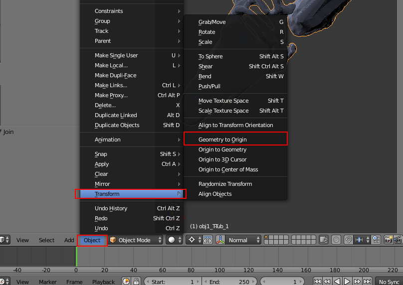
6. To simplify future manipulation let’s center the model about the origin.

   • select Object near the bottom left of the 3D window, then select transform, then select Geometry to Origin.

     

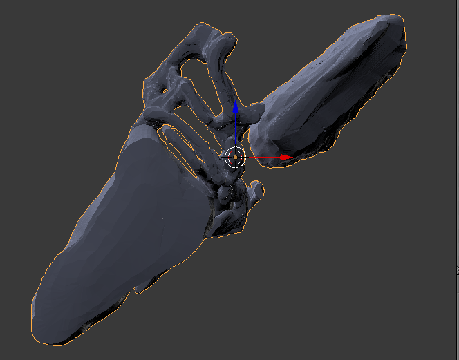
7. Set the origin again just as before with the Period on the Numpad then to set the focus to the front of the object press 1 on the Numpad. Your 3D View window should now look something like the following.

   

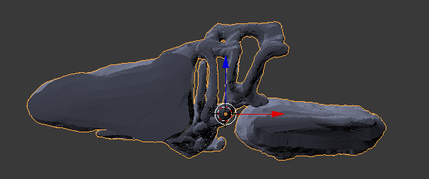
8. Let’s now align the model so that the long axis is horizontal.

   • Rotate about the y-axis by 45 degrees to line up the model horizontally, by hitting r, y, and 45.

     

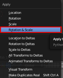
9. Save this state as the object’s default rotation and scale via one of two ways.

   • Select Object near the bottom left of the window, then select Apply, then select Rotation and Scale.

     

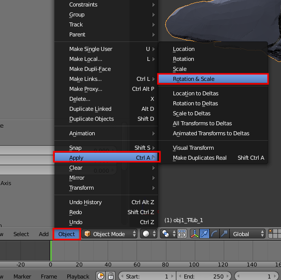
   • Or you can press Ctrl+a and then select Rotation and Scale.

     

10. CHECKPOINT: Let’s save our work now as: tt-sr-mit.imp_obj.blend. Note that if something goes awry, you can always close Blender and reopen at this checkpoint! Checkpoints are also available online.

Analyze Mesh, Clean-up, and Repeat

1. BlendGAMer has a mesh analysis report which can help you to inspect the mesh’s quality.

   • In the Tool Shelf select the GAMer tab and go to the Mesh Quality Reporting panel. Click the Generate Mesh Report button. You should see a number of statistics appear.

     

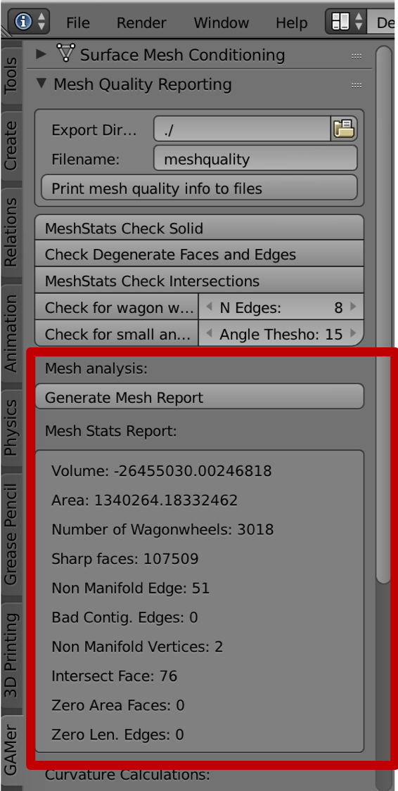
     Here is a summary of the report features:

     • Volume: The volume of the geometry

     • Area: The surface area of the mesh

     • Number of Wagonwheels: The number of vertices with adjacency greater than the setting above (default: 8)

     • Sharp faces: High aspect ratio triangles with an angle less than the threshold set above (default: 15)

     • Non Manifold Edges: Number of edges not connected to two faces

     • Bad Contiguous Edges: Edges across which the normal orientation of the mesh is inconsistent

     • Non Manifold Vertices: Vertices participating in a non-manifold feature

     • Intersecting Face: Faces which intersect with another

     • Zero Area Faces: Faces with zero area

     • Zero Length Edges: Edges with zero length

     We can see that this initial mesh has a number of issues. Most importantly, there are a number of non-manifold edges and vertices.

     Note

     Manifold geometry is essentially geometry which can exist in the real world. For some pragmatic examples of non-manifold geometry please consult the following stackexchange.

2. Let’s start by cleaning up these regions of non-manifold topology. The other issues, including wagonwheels, sharp faces, and intersections will be resolved by BlendGAMer mesh conditioning.

   • First engage Edit Mode [Tab] and while having the cursor in the 3D view window deselect everything by pressing [a].

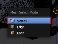
   • Hit Ctrl-Tab and select Vertex select mode.

     

   • Click Select near the bottom left of the window, then click Select All By Trait, then click Non Manifold.

     

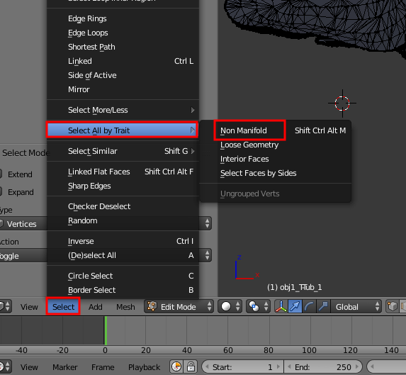
     Or you could press [Shift+Ctrl+Alt+m] as a shortcut. This highlights all the regions of non-manifold topologies.

     

3. Conveniently non-manifoldness is a problem in the animation industry (it tends to cause problems with raytracing among other things). Thus, Blender has some built-in tools to help resolve non-manifoldness.

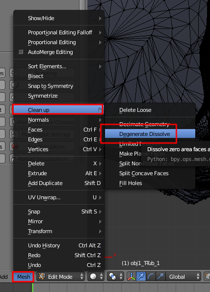
   • First, Select All by pressing [a] with the cursor in the 3D view window, then near the botttom left of the 3D window select Mesh, then Clean up, then Degenerate and finally Dissolve. This function will take care of several cases of bad geometry: edges with no length, faces with no area, or face corners with no area. It does so by deleting vertices and edges it thinks don’t make sense.

     

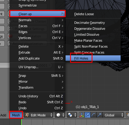
   • This will leave some holes in the mesh. We can automatically fill the holes by again selecting Mesh near the bottom left of the 3D window, then Clean up, then Fill Holes.

     

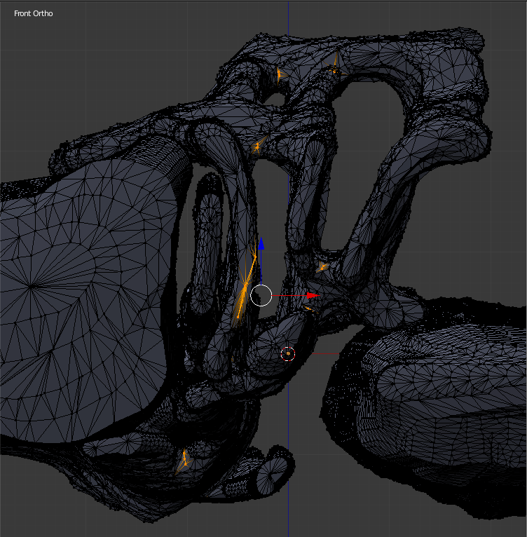
   • Let’s check to see if all of the issues have been resolved. Deselect everything by pressing [a] with the cursor in the 3D window again and then near the botttom left of the 3D window click Select, then Select All By Trait, then Non Manifold. Or we could use [Shift+Ctrl+Alt+m] as a shortcut.

   • We see that the mesh has been improved but there remains one region with an issue.

     

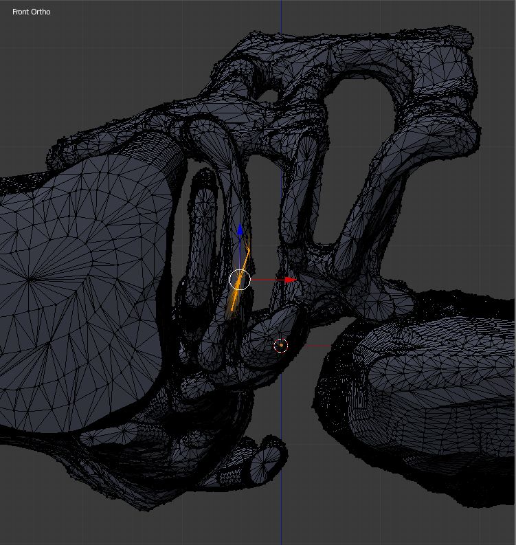
4. We can zoom in on the selected region by again having the cursor in the 3D window and then on the Numpad select the Period.

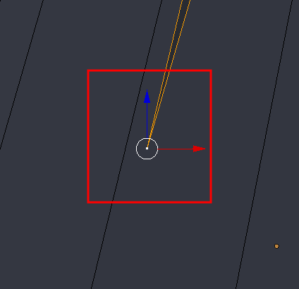
   • Let’s delete the dangling vertex. First Deselect everything [a] then select the culprit vertex [RMB click] (Note this can be difficult to find so make sure you have the view outside the object and not inside) and delete [x] and choose Vertices.

   • Normal view of the culprit vertx

     

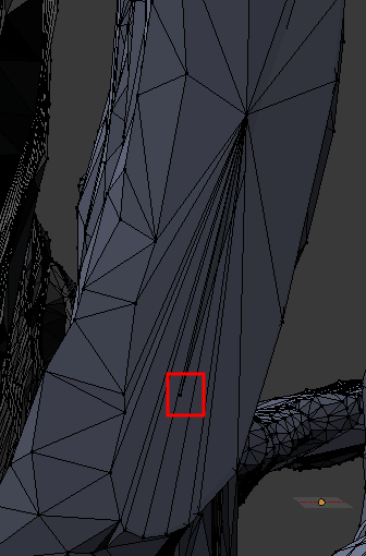
   • Close up of the culprit vertex

     

5. Once again let’s take a look to see if there are any residual problems. In Edit Mode [Tab], click Select, then Select All By Trait, then Non Manifold. Or we could use [Shift+Ctrl+Alt+m] as a shortcut. At this point your mesh should have no more issues.

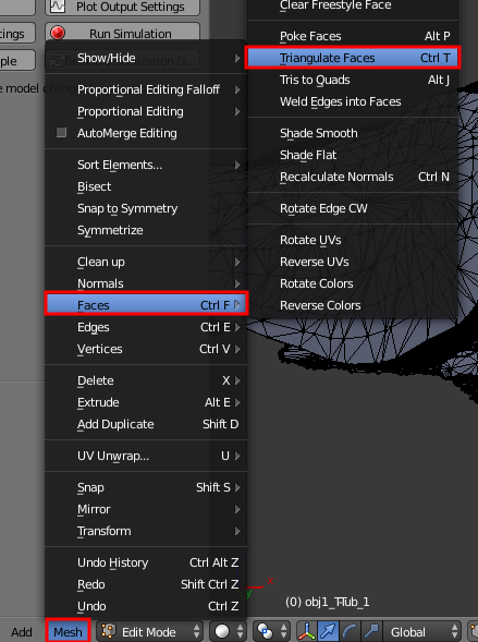
6. Recall that the degenerate dissolve function deleted some vertices and edges. In some cases, when the holes are filled, the polygons may no longer be triangular.

   • To re-triangulate, select everything [a] and choose Mesh, then Faces, then Triangulate. Or [Ctrl+t] as a shortcut.

     

7. Our mesh is starting to look pretty good! Let’s re-run the mesh quality report. Note that the volume is reporting a negative number. This is because the normals of the mesh are currently facing the wrong way. You can follow these steps to fix this issue. Alternatively, BlendGAMer can also automatically detect this problem and flip the normals automatically in later steps.

   • Select Mesh, then Normals, then Recalculate Outside or you could use [Ctrl+n] as a shortcut.

   • Once the normals are flipped the volume and surface area should report 2.6457e7 and 1.34e6 respectively.

8. CHECKPOINT: Save your progress to: tt-sr-mit.clean.blend.

Using BlendGAMer to Condition the Mesh

We are now ready to begin surface mesh refinement with GAMer.

1. Go to the GAMer tab on the left side of Blender. Click on the Surface Mesh Conditioning subpanel.

   

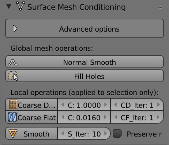
   The subpanel provides several functions as follows:

   • Normal Smooth: smooths surface roughness using a feature-preserving normal averaging algorithm.

   • Fill Holes: Triangulates holes in the mesh.

   The following tools are only available in Edit Mode and operate on selected vertices only.

   • Coarse Dense: reduces the number of triangles in densely triangulated portions of the mesh.

   • Coarse Flat: reduces the number of triangles in flat regions of the mesh.

   • Smooth: improves the aspect ratio of triangles by maximizing angles. It does so by flipping edges moving vertices based on angle and the local structure tensor.

2. In Edit Mode [Tab] with the full model selected, perform the following operations in order. After each step the approximate number of vertices remaining is given.

   • Smooth: S_Iter = 15 (~73K vertices)

   • Coarse Dense: CD_R, 1.5; CD_Iter, 5 (~35K vertices)

   • Smooth: S_Iter, 15

   • Coarse Dense: CD_R, 1; CD_Iter, 5 (~23K vertices)

   • Smooth: S_Iter, 20

   • Normal Smooth

3. Returning to the Mesh Quality Reporting generate a new report. Most of the issues previously reported should be resolved at this point. At this point continue to Smooth the mesh until there are no sharp faces reported. Note that you can change the threshold for sharp faces by changing the Angle Threshold above.

   Note

   If there are specific regions of your mesh where there are persistent intersecting faces, in Edit Mode you can select them from the Mesh Stats Report by clicking the corresponding button. With these regions selected, you can apply iterations of smooth directly to these regions.

4. The mesh is starting to look pretty good. Rerun the mesh quality report and note the slightly smaller surface area but similar volume around 1.13e6 and 2.64e7 respectively.

5. CHECKPOINT: Save your progress to: tt-sr-mit.gamer_proc_1.blend

Add Boundary Box

Now that we have a reasonable surface mesh of the organelle membranes. If we want to model diffusion in the cytosol we must invert the domain to represent the cytosol. First, we want to place a boundary box around the features to represent the cytosolic domain. In the next section we will use a mesh boolean operation to perform the inversion.

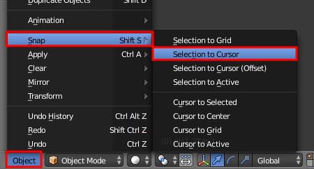
1. First center the 3D cursor to the center. In Object Mode, select Object, then Snap, then Cursor to Center or you could use [Shift+s and select Cursor to Center] as a shortcut.

   

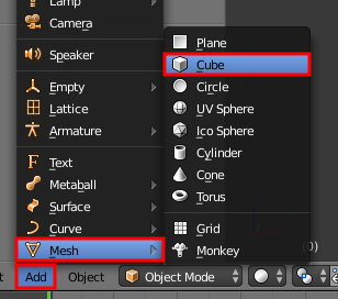
2. Next, with the cursor at the origin still, add a cube at the position of the 3D cursor. Add a cube mesh object, select Add, then Mesh, then Cube. Or you could use [Shift+a and select Mesh, then Cube] as a shortcut.

   

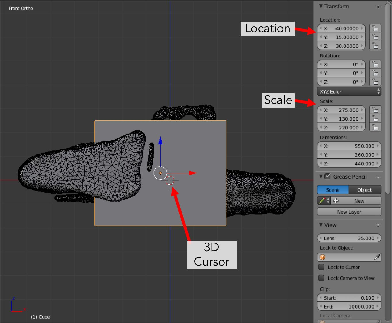
3. In Object mode [Tab], let’s scale and translate the bounding box to where we want it. Recall that the Properties panel can be summoned with [n].

   • Location (-40, 15, 30)

   • Scale (275, 130, 220)

1. The cube is currently a quadrilateral mesh. We need to convert it to a triangular mesh.

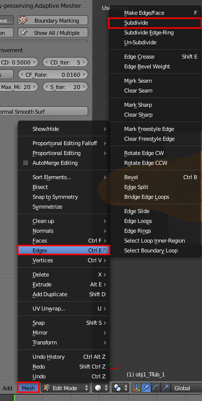
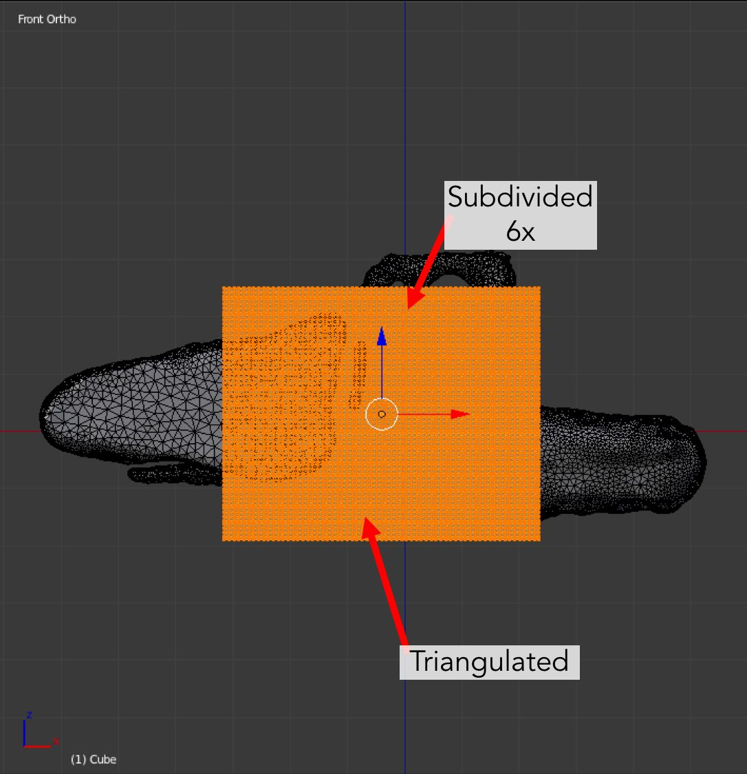
   • In Edit Mode [Tab] triangulate by selecting Mesh, then Faces, then Triangulate Faces. Or you could use [Ctrl+t] as a shortcut.

2. The cube currently has too few triangles. If we performed the boolean mesh subtraction with this mesh, the post-triangulated result will contain may high aspect ratio triangles. To avoid this we can subdivide the cube domain to improve mesh resolution.

   • In Edit Mode [Tab] with the cube selected, select Mesh, then Edges, then Subdivide a total of six times. Alternatively you can use [w and select Subdivide] as a shortcut.

   

3. Return to Object Mode [Tab].

   

4. CHECKPOINT: Save your progress to: tt-sr-mit.with_cube.blend

Using Boolean Modifier

To get the a representation of the cytosolic volume, we must subtract our features from the cube mesh.

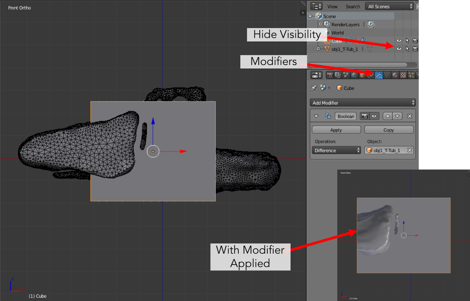
1. While in Object Mode [Tab], with the cube selected, go to the Modifier tab of the Properties Panel and hit Add Modifier, Generate: Boolean, Operation: Difference, Object: obj1_T-Tub_1 and Apply the modifier.

   • In the Outliner click on the eye to hide obj1_T-tub_1.

   • With the cube selected, apply the current rotation and scale transform. Select Object, then Apply, Rotation and Scale, or use [Ctrl+a and select Rotation and Scale]

   • Apply the current location transform. Select Object, then Apply, then Location or use [Ctrl+a, Location].

   • If you would like to show the edges, go to the Object Properties and select Wire and Draw all Edges.

   

2. CHECKPOINT: Save your progress to: tt-sr-mit.boolean.blend

Refine Cube with GAMer

Once again, we have a surface mesh to refine.

1. First let’s verify that there are no elements causing non-manifoldness.

   • In Edit Mode [Tab], switch to Vertex select mode.

   • Deselect everything [a].

   • Next, we can click Select, then Select All By Trait, then Non Manifold, or [Shift+Ctrl+Alt+m]. Nothing should be selected. If there are some issues, try performing Degenerate Dissolve followed by Fill Holes.

2. After the boolean operation, the mesh is no longer triangulated. We can triangulate as before:

   • In Edit Mode [Tab], Select All [a] , then select Mesh, then Faces, then Triangulate Faces or [Ctrl+t].

3. CHECKPOINT: Save your progress to: tt-sr-mit.boolean_clean.blend

4. Let’s begin surface refinement using GAMer:

   • In Edit Mode [Tab] with the cube selected, perform the following operations in order. After each step the approximate number of vertices remaining is given.

   • Smooth: S_Iter = 10 (~38K vertices)

   • Coarse Dense: CD_R = 0.75, CD_Iter = 10 (~34K vertices)

   • Coarse Flat: CF_Rate = 0.016, CF_Iter = 1 (~19K vertices)

   • Smooth: S_Iter = 10

   • Coarse Dense: CD_R = 0.1, CD_Iter = 10 (~18K vertices)

   • Smooth: S_Iter = 20

   • Normal Smooth

5. Generate a new mesh report. Note the slightly smaller surface area but similar volume.

6. CHECKPOINT: Save your progress to: tt-sr-mit.gamer_proc_2.blend Now we’re ready to add boundaries and associated boundary markers to the mesh!

Adding Cytosolic Boundary

Now that the mesh is in good shape, it’s time to mark boundaries for future use assigning boundary conditions.

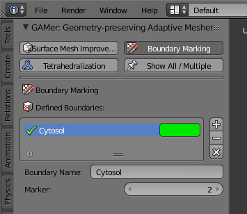
1. Return to the GAMer tab and select the Boundary Marking tool and add a new boundary.

   • Add a new boundary by clicking the + button. By clicking on the color swatch, you can select the color you wish to represent the Cytosol. The color only serves as a visual aid to help you mark. Set the color to green.

   • Change the name of the boundary to Cytosol.

     

2. Enter Edit Mode [Tab] and choose Face select mode and begin selecting all faces of the cytosol. Clicking each face is very arduous! For larger surfaces, you may elect to select using the Circle Select tool [c] or the Border Select tool [b]. Use “Assign” to assign selected faces to boundary. You can assign as you go or all together at the end. Note, it can sometimes be very helpful to hide all selected faces using [h], or hide all unselected faces using [Shift+h]. You can unhide everything using [Alt+h].

   • In the next steps, we’ll be using the Border Select tool [b].

   • Turn off the option: Limit selection to visible.

   • Front-View [numpad 1].

   • Select faces of Cytosol. Use Border Select tool [b] to select the profile of each side.

   • Top-View [numpad 7].

   • Select additional faces of Cytosol. Use Border Select tool [b] to select the profile of remaining sides.

   • Hide all unselected [Shift+h]. You may notice that some triangles from the organelle membranes may have been selected. We will fix this next by selecting linked triangles.

   • Deselect all [a]

   • Select one triangle, click [RMB].

   • Select Linked [Ctrl+l]

   • Hide All Deselected [Shift+h]

   • Use Assign to assign selected faces to boundary.

   • Turn on option: Limit selection to visible.

   • Unhide All [Alt+h]

   • Deselect all [a]

3. CHECKPOINT: Save your progress to: tt-sr-mit.cytosol.blend

Adding Other Boundaries

1. When you are finished marking the cytosol, make the following changes

   • Select and hide faces marked as Cytosol [h].

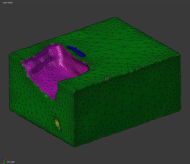
   • Add a new boundary named Mitochondria and set the color to magenta.

   • Select one face on each mitochondria [Shift+RMB] and Select Linked [Ctrl+l]

   • Use Assign to assign the selected faces to be in the mitochondria.

   • When finished, hide the mitochondria [h] and proceed with marking the t-tubule (T-tubule, Set color to blue) and sarcoplasmic reticulum (Sarcoplasmic Reticulum, Set color to yellow).

2. Set the marker values of each boundary as follows:

   • Cytosol: 10

   • Mitochondria: 20

   • T-tubule: 30

   • Sarcoplasmic Reticulum: 40

   

3. CHECKPOINT: Save your progress to: tt-sr-mit.all_marked.blend

Tetrahedralization

Next we tetrahedralize this domain.

1. In Object Mode, select the boundary marked mesh and click + in the Tetrahedralization subpanel to add the domain to be tetrahedralized.

2. Next, expand the tetrahedralization setting and set the export directory, filename prefix, and check the outputs you would like. We recommend checking Paraview which will enable you to view the resulting tetrahedral mesh in Paraview.

3. Click tetrahedralize!