Solving a diffusion PDE on a GAMer mesh using FEniCS
This tutorial will walk you through the process of setting up and solving a diffusion partial differential equation (PDE) using a mesh imported from GAMer into FEniCS
[1]:
import pygamer
import math
Generating the mesh using GAMer
[2]:
# generate the surface mesh for a cube
smesh = pygamer.surfacemesh.cube(5)

# Mark sides of the face to use later for boundary conditions
for fid in smesh.faceIDs:
    indices = fid.indices()
    z_coords = [smesh.getVertex([idx]).data().position[2] for idx in list(indices)]
    if all([z==1 for z in z_coords]):
        fid.data().marker = 2
    elif all([z==-1 for z in z_coords]):
        fid.data().marker = 3
    else:
        fid.data().marker = 4

# construct the volumetric mesh
vmesh = pygamer.makeTetMesh([smesh], "q1.1/15O10/2ACVY")

# write volumetric mesh into dolfin readable format
pygamer.writeDolfin('outputTetMesh.xml', vmesh)
pygamer.writeVTK('outputTetMesh.vtk', vmesh)
Number of vertices: 1538
Number of Faces: 3072
Number of Regions: 1
Number of Holes: 0
Region point: Tensor({0}:-0.875; {1}:0.333333; {2}:-0.333333)
Setup the model problem in FEniCS
Model problem: strong formulation
We will model diffusion in a \(2 \times 2 \times 2\) cube with an exponentially decaying source term centered at the origin, an influx boundary condition at the \(z=1\) surface, an outflux boundary condition at the \(z=-1\) surface, and a \(u=0\) Dirichlet boundary condition on the four other sides of the cube.
Find \(u(\mathbf{x},t)\) such that
where \(f\) is the source term, \(f(\mathbf{x}) = 32 - e^{||\mathbf{x}||}\), \(D\) is the diffusion coefficient, \(j_\text{in}\) and \(j_\text{out}\) are the influx/outflux rates for the Neumann boundary conditions, and \(u_0\) is the initial condition.
[1]:
import dolfin as d

# Model parameters
D    = 1 # diffusion coefficient
u0   = d.Constant(0.001) # initial condition
dt   = 0.1 # time step size
T    = 1.0 # final time
jin  = 10.0 # influx rate
jout = -50.0 # outflux rate
dist = d.Expression("sqrt(pow(x[0],2) + pow(x[1],2) + pow(x[2],2))", degree=1)
f    = d.Expression("32 - exp(dist)", dist=dist, degree=1) # source term
t    = 0.0 # current time

numsteps = round(T/dt)
Model problem: weak/variational formulation
The finite element method uses a variational formulation of the PDE which allows us to search for solutions from a larger function space. Equations input into FEniCS are done so through their variational formulation; we will now show how to convert our problem into a valid FEniCS input.
First we multiply the governing PDE by a test function, \(v\), coming from a function space \(V\), integrate over the domain and apply the divergence theorem to obtain the following variational formulation:
We discretize the time-derivative with a backward Euler scheme due to its simplicity and unconditional stability properties
where \(u_n\) represents the (known) solution computed at the previous timestep. We further simplify the variational formulation by inserting the Neumann boundary conditions and using the shorthand notation where \(\langle \cdot , \cdot \rangle\) represents the inner-product over \(\Omega\) and \(\langle \cdot , \cdot \rangle_{\partial\Omega_\text{in}}\) represents the inner-product on the boundary \(\partial\Omega_\text{in}\). Terms are separated onto the left or right hand sides by their dependence on \(u\):
Notice that since \(u_n\) is a known value it is not dependent on the unknown, \(u\), and therefore is placed on the right hand side. Also, since \(D(\mathbf{n}\cdot \nabla u)=0\) on the no-flux boundary those terms drop out of the variational formulation.
In the abstract form this is written as,
where \(a(u,v)\) is a bilinear form and \(L(v)\) is a linear functional. Note that the Dirichlet boundary condition does not appear in the variational form and therefore must be enforced separately.
[2]:
# Import the mesh and construct a linear Lagrange function space over the mesh
dolfin_mesh = d.Mesh('outputTetMesh.xml')
V = d.FunctionSpace(dolfin_mesh,'P',1)
[3]:
# Define trial and test functions
u = d.TrialFunction(V)
v = d.TestFunction(V)
# Known solution corresponding to previous timestep. Initialize with initial condition
un = d.interpolate(u0,V)
[4]:
# Earlier we marked faces on the influx boundary with 2 and faces on the outflux boundaries as 3

# define integration domains
face_dimension = 2 # we marked faces which have a topological dimension of 2
meshBoundary = d.MeshFunction("size_t",dolfin_mesh,face_dimension,dolfin_mesh.domains())
dx = d.Measure('dx',domain=dolfin_mesh)
ds = d.Measure('ds',domain=dolfin_mesh,subdomain_data=meshBoundary)
[5]:
# define bilinear and linear forms
a = u*v*dx + D*dt*d.inner(d.grad(u),d.grad(v))*dx
L = dt*f*v*dx + dt*jin*v*ds(2) + dt*jout*v*ds(3) + un*v*dx
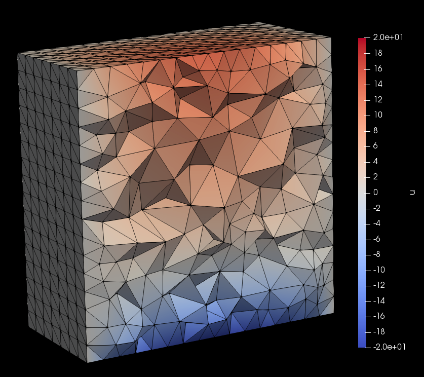
Solve and store solution
Solutions are saved in the \(\texttt{.vtk}\) format and can be visualized using software such as Paraview
[6]:
filename = 'solution/dolfinOut.pvd'
vtkfile = d.File(filename)

# store the initial condition
u = d.Function(V)
un.rename("u", "solution")
u.rename("u", "solution")
vtkfile << (un,t)

bc = d.DirichletBC(V,d.Constant(0),meshBoundary,4)

# Main loop
for idx in range(numsteps):
    # step forward in time
    t += dt

    d.solve(a==L,u,bcs=bc)

    # save solution to file
    vtkfile << (u,t)

    # assign just computed solution to un
    un.assign(u)

    print('Time step %d complete ...' % int(idx+1))
Time step 1 complete ...
Time step 2 complete ...
Time step 3 complete ...
Time step 4 complete ...
Time step 5 complete ...
Time step 6 complete ...
Time step 7 complete ...
Time step 8 complete ...
Time step 9 complete ...
Time step 10 complete ...
[ ]: